In this blog, we explore some of the ways that simulated FASTQ data differs from real reads generated by a sequencer on a true human genome. We conducted this analysis through the lens of the development of a new strategy for discovering copy number variants. The differences we encountered illustrated some of the challenges of using simulated data. We used these differences to analyze the quality of reference genomes themselves and compare GRCh37 with GRCh38.
Introduction
Both the development and assessment of any new method start from well-understood initial datasets. When available, well-characterized exemplar datasets (for example, the Genome in a Bottle genomes for SNP and Indel calling) are powerful resources. However, in some cases, creating simulated datasets with understood and controlled properties is the only way to develop.
In genomics, many simulation methods have been written specifically for this purpose, including Mason, WGSIM, and DWGSIM for FASTQ generation and a myriad of others for small variants, structural variants, gene expression, and metagenomes.At the same time, it is very challenging to create a simulation which fully captures all of the biases in real systems. A FASTQ simulator must model the biases in GC sequence context, the base, insertion, and deletion error profile, and the insert size distribution. Further, it must capture how each term interacts with the others.
In working with simulated data to form a baseline, we encountered an additional issue in FASTQ simulation, which arise not because the simulators imperfectly model sequencing, but because the reference genome itself is still imperfect. This leads to regions where the sequence content is significantly over- or under-represented relative to sequence of a human from a real sequencer.
How Incompleteness of the Reference Might Impact Simulations
Most genomics analyses are conducted relative to reference genomes. Having a reference makes analysis much easier computationally. It also serves as a shared yardstick against which other samples can be measured, creating a common vocabulary for gene and variant positions and content. Reference genomes are hard to assemble because many parts of the genome look similar to each other (such as centromeres, telomeres, mobile elements, and segmental duplications).
The human reference genome is continually evolving, with the most recent version being GRCh38. However, the last version was produced in 2013, before powerful long-range technologies like PacBio, 10X, Oxford Nanopore, Dovetail, Phase, BioNano, and Nabsys started to hit full stride and which could complement the strong and intensive BAC by BAC approach.
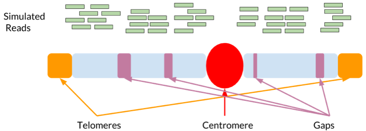
The above figure contains a highly simplified schematic of a chromosome. The purple, red, and orange regions represent types of areas where the reference sequence is likely incomplete. The green simulated reads demonstrate that near these regions the simulation only samples partially.
Sashimi – a Method for Copy Number Variation Leveraging Salmon
To frame our work, we must give an overview for a new method we have been developing to discover copy number variations (CNV). Here we provide a high-level overview of Sashimi. In a future blog post, we will delve into methods and benchmarks in greater detail.
Sashimi is a method that is built on top of Salmon, which performs RNA-Seq quantification. The central idea behind Sashimi is that detecting the number of copies of a segment of DNA is conceptually similar to detecting the copies of RNA. Salmon models and corrects for a number of complex factors that make structural variant calling hard (bias GC sampling and smart weighting of ambiguous support), and is both rapid and learns these weights directly from the data.
Salmon produces a normalized value to quantify the number of copies for a sequence represented in the data as Transcripts per Million (TPM), which in our case is instead an estimate of the DNA copies. In Sashimi, we index the genome into 500bp bins. We run Salmon to determine TPM counts for each segment. We smooth and normalize this signal to identify CNVs.
We simulated deletion events in the reference with SURVIVOR and simulated reads with Mason. To compare with real data, we used a set of candidate truth structural variants (v0.6) generated by Genome in a Bottle for HG002 and a 35X HiSeqX sample from the precisionFDA Truth Challenge.
Differences in TPM Calculated by Salmon from Simulated and Real FASTQ Data
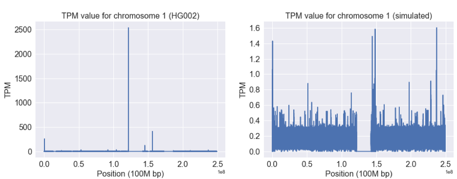
The left figure above shows the TPM value from real data across chromosome 1, while the right shows the same values for the simulated data. Note the difference in the y-axes between the two: the real data has a maximum value more than 1000 times that of the simulated data. The regions with 0 TPM are scaffold sequence (NNNNN…).
Why are these plots so different? The region 5’ to the centromere has a number of sequence repeats. As a result, there will be many reads with this sequence. Salmon has a clever approach to manage reads that could support multiple transcripts: it assigns them to the different models in a weighted manner based on the probability to support them.
Since the reference is incomplete, the number of reads in a real sample will proportionally be much higher than the regions for Salmon to divide them. Thus in a real sample this will cause coverage to pile up in regions with sequences that resemble the missing components. Because Mason can only consider the reference as correct, it simulates data in proportion to the incomplete reference.
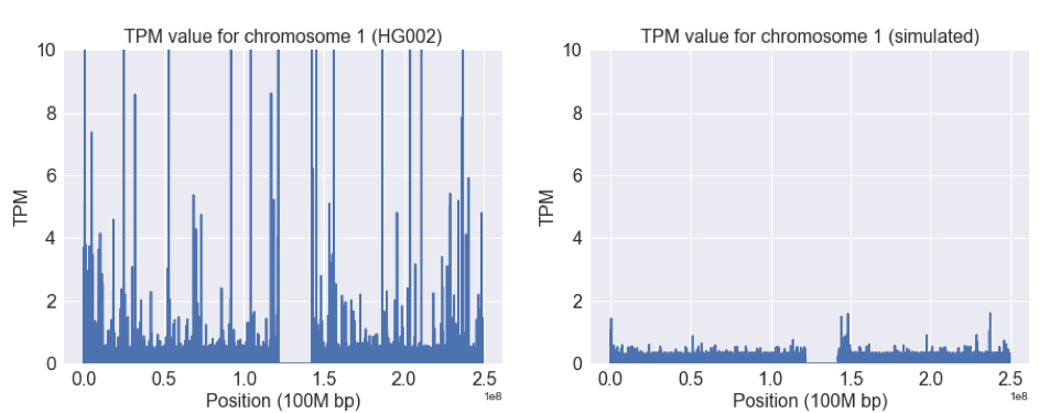
Setting the TPM cap to 10 allows us to see a host of other regions with a similar effect:
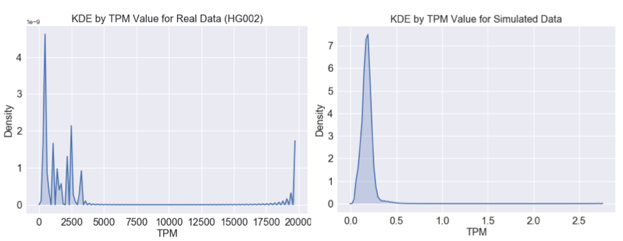
The figures below show the density for TPM values calculated for real and simulated data across the genome binned by TPM. The peaks at the right extreme TPM show the same effect.
In Regions Represented Well by the Reference, Differences Between Simulated and Read Data are Detectable
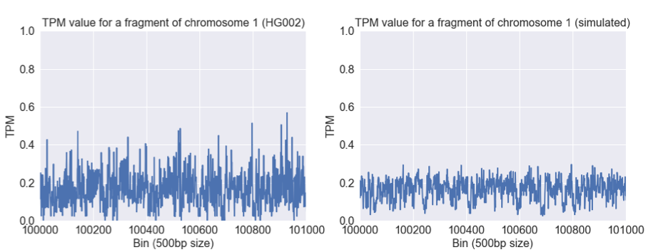
We can constrain our analyses to regions outside of these extreme peaks. When we do so, it is still possible to detect the differences between real and simulated data when viewed from our lens of Salmon TPM.
The TPM values are much more consistent in this region (most genome regions look like this), and both have a mean of around 0.2 TPM. However, there is more variability in the real data. This likely reflects some sampling bias (e.g. GC or sequence context) that is not captured in the simulation.
Measures of Precision and Recall for a Method Can Be Very Different in Simulated Data
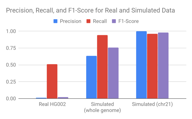
Unfortunately, this sort of variability present in real data but not simulated data is exactly the sort of thing that makes CNV calling much more difficult. We tried a variety of smoothing and machine learning to call CNV events. The performance we could achieve in simulated data was very different from the performance we could achieve on the Genome in a Bottle set.
If we took the accuracy of Sashimi only on simulated data and compared it to our benchmarks of other CNV methods on Genome in a Bottle, we would conclude Sashimi is best in class. If we constrained the simulation to only chromosome 21, we would conclude the problem to be virtually solved.
Going from real data to simulated and then from simulated to only chromosome 21 simplifies the problem we are trying to solve in artificial ways – because the simulation doesn’t reflect key properties relevant to CNV calling. The chromosome21 sample is easier still because it removes the complexity of interchromosomal segmental duplications.
Why This Affects Processes Like CNV Calling or SNP and Indel Calling
In a real sample, the incompleteness of the reference will cause coverage to pile up in regions with sequences that resemble the missing components. These mismapped reads may have sequence divergence which falsely looks like SNP and Indel signal to variant callers. Common signals for structural variant and CNV callers (reads mapped in proper pairs, average depth, insert size) will also be increased in these sorts of regions. The GC variability observed will also cause fluctuation in coverage. When using simulated data, these features will not be present.
Because of the way structural variant and CNV callers work, they will likely be more affected than SNP and Indel callers. For SNP and Indel calling, some of this may explain observations by Heng Li on difficulties calling in high coverage regions, and the recommendation to filter low-complexity regions.
The Difference Between Simulation and Reality Allows Us to Assess Improvements in the Reference Genome
All of the analyses conducted so far have been on the GRCh37 reference genome. Instead of measuring samples by comparing to the reference, we can measure the reference by comparing to the samples.
The figure below shows the same graph for real HG002 when applying Salmon with GRCh37 (hs37d5 version) or GRCh38 (with decoys but not ALT). Note the scale difference between the two figures. Many of the gaps have been narrowed.
Here is the same, but with a cap of 10 TPM, showing improvement in hg38 beyond just the most impacted regions.
The kernel density estimator plot quantifies the overall reduction of incompleteness in a genome-wide manner between GRCh37 and GRCh38 (again note the difference in TPM scales):
We presume that, as the human reference genome continues to improve, these artifacts in the Salmon quantification will decrease. It should also be possible to use this measure to assess regions that are incomplete in non-human references with varying degrees of polish, and to automatically estimate the approximate sizes of gaps.
There is additional complexity for not discussed here – the current reference is a “monoploid” representation and so inherently departs from any of us a diploid humans. This limitation may be improved over time as more high-quality references become available representing diverse ancestries (any two of which could be combined for the purposes of simulating a diploid).
Conclusion
We hope that we have provided insight into some of the differences that may arise in using simulated data, particularly FASTQs. We expect this effect to be relatively strong with regards to CNV calling. We think this phenomenon will likely affect the use of simulated data for SNP and Indel calling to a lesser extent, with a greater impact felt in regions of low sequence complexity and those near reference gaps.
We hope that this method could be promising for assessing reference genomes, and we hope this has given some insight into potential improvements in GRCh38.
Although these issues have made it difficult to build Sashimi as a full, genome-wide CNV caller, we believe that the approach will be viable for detecting large deletions, for modeling CNVs on a gene-by-gene manner, and for confirming events. We hope to detail Sashimi for this use case in a later post.
Final Note About the Authors:
DNAnexus has teams of software engineers, who build and maintain the infrastructure, web GUI, security systems, and developer tools that power the DNAnexus Platform. We also have teams of bioinformaticians who develop applications on DNAnexus, help customers deploy their workflows, and represent DNAnexus in the scientific community.
DNAnexus has a commitment to the development and growth of our employees and to connect with the scientific community. As a part of that, we have the option for both scientists and engineers to take 10% of their time (currently Friday afternoon) to work collaboratively on projects.
The authors of this work, Aleksandra (Ola) Zalcman and Calvin Bao are software engineers at DNAnexus. The figures and analysis you see here are a small fraction of the body of work that contains the various ideas, pivots, false starts, and side investigations that come with developing a new method. Ola, as the lead author in this work, has shown great dedication in continuing to push the work forward, experiment by experiment, every Friday.
This work speaks to the fact that science isn’t something you need a specific pedigree or credential to do – science only requires you to bring curiosity, collaboration, rigor, and effort. Being able to work in an environment full of such sharp, collaborative people with different backgrounds and expertise is one of the best things about working at DNAnexus.
We thank Deanna Church of 10X Genomics and John Didion of DNAnexus for helpful comments, Samantha Zarate for technical editing, and the authors of Salmon: Rob Patro, Geet Duggal, Michael Love, Rafael Irizarry, and Carl Kingsford.
Methods and Commands:
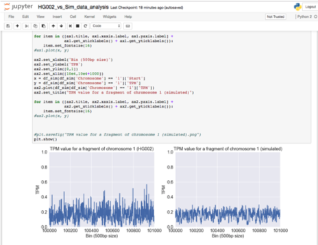 A Jupyter notebook with the analysis and data conducted in this blog can be downloaded at this link (note that this is a 500 MB download).
The applets and index files are available in this public DNAnexus project (anyone with an account can access this project) from the link above.
The commands and parameters used to generate the reads, run Salmon, and simulate the events:
Generate Salmon Index
Split the reference fasta into 500bp contigs. Index with:
salmon index -t GRCh38.no_alt_analysis_set.all.500base_chunk.fa -i GRCh38.no_alt_analysis_set.all.500base_chunk_k31_index -p 32 –type quasi -k 31
Simulate Reads with Mason:
mason_simulator -ir ${REF} –seed ${SEED} -o mason.R1.fastq -or mason.R2.fastq –illumina-read-length 150 -n ${READ_NUMBER} –read-name-prefix ${PREFIX} –illumina-prob-insert 0.00005 –illumina-prob-deletion 0.00005
Quantify with Salmon:
salmon quant -i GRCh38.no_alt_analysis_set.all.500base_chunk_k31_index -l IU -1 HG002NA2438550x_1.70_percent.fastq -2 HG002NA2438550x_2.70_percent.fastq -o HG002NA2438550x__quant -k 31 -p 32 –seqBias –numBiasSamples 1000000 –posBias –gcBias
Simulate CNV Events with SURVIVOR:
SURVIVOR 1 ${REF} parameters.txt 0 0 ${PREFIX}
The parameter file can be downloaded from the link above.




.png)
.png)
.png)