

Working at DNAnexus has given me the opportunity to explore a bunch of AI/machine learning developments, especially those that pertain to biology. This will be the first in a series of blog posts where I will explore new and/or relevant ideas in the field.
One of the most recent advances in the field to make a splash comes from Stokes et al., where they developed a deep learning method to discover antibiotics1. The first antibiotics were discovered serendipitously by identifying the active ingredient in observations of microorganism growth inhibition, as was the case with penicillin. In the last several decades, the rate at which new classes of antibiotics have been discovered dropped considerably2. Large-scale screening has had limited, if any, success. Hence, an in silico approach as described by the authors could significantly speed up the discovery process. Using their deep learning method, the authors identified a promising new antibiotic, halicin (formerly known as SU-3327), as well as eight other potential antibiotic candidates.
In this blog post, I will go over the deep learning algorithm they developed to solve this problem. I will also demonstrate my experiences replicating their results with the JupyterLab Notebook on the DNAnexus Platform and share my thoughts on where I see this field going.
What is molecular property prediction?
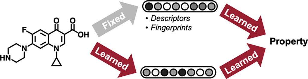
Figure 1. Two different approaches to molecular property prediction. Each method differs in how they achieve a feature vector representation of a molecule.
The main idea behind applying machine learning to enable drug discovery is to automate the prioritization of molecules with desired properties for downstream experimental verification. This is achieved by training models on datasets of molecules with known molecular properties so that the models can generalize to molecules not found in the training set. Molecular property prediction is one of the oldest cheminformatic tasks. In simple terms, the molecular property prediction problem can be stated as follows: given an input molecule, x, and its property label, y (e.g. toxicity, thermodynamic property, etc), find a function mapping, f, such that the error between f(x) and y is minimized. The molecule, x, can have an arbitrary number of atoms and bonds, but the size of y remains fixed (often a single binary or real-valued number), so the function mapping, f, must include a preprocessing step to convert the molecule into a constant length feature vector. Two methods for achieving this constant length feature representation have achieved considerable success: rule-based algorithms that convert molecules into fixed-length fingerprints and graph convolutional neural networks that construct a learned molecular representation by operating on the graph structure of the molecule (Figure 1).
Morgan fingerprints
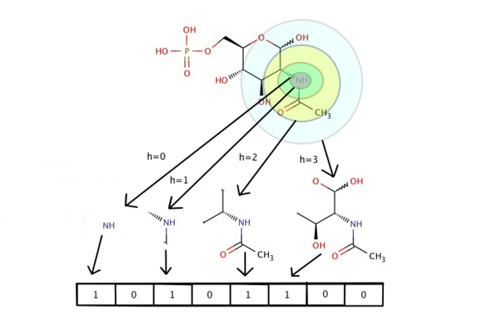
Figure 2. The Morgan algorithm converts a single molecule into a fixed number of binary bits (e.g. 2048). Each bit corresponds to the presence/absence of chemical substructures up to a specified radius (e.g. 2). (source: https://towardsdatascience.com/https-medium-com-aishwaryajadhav-applications-of-graph-neural-networks-1420576be574)
Molecular fingerprints are computed using the Morgan algorithm3. The algorithm for generating these fingerprints is pretty complicated, so I won’t go over it in complete detail here, but I present a brief illustrative explanation of how it works in Figure 2. These fingerprints, ideally, satisfy two conditions:
- Provide a unique representation for each molecule (i.e. prevent collisions, similar to hashing functions).
- Molecules with similar chemical structures should yield similar fingerprint representations as measured by the Tanimoto (or Jaccard) coefficient.
Since fingerprint similarities can be measured by the Tanimoto coefficient, they lend themselves quite well to the T-SNE algorithm for visualization. Through visualization, it’s easy to see how similar the novel antibiotic halicin is to other drugs (Figure 3).
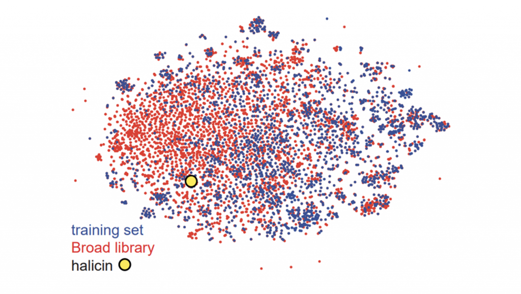
Figure 3. T-SNE visualization using Morgan fingerprints for all molecules in the study’s internal training set (n=2,560) and the Broad’s Drug Repurposing Hub (n=6,111). Halicin is labeled with a yellow circle.
A simple, yet effective approach for predicting molecular properties is to apply a feedforward neural network directly on the fingerprints (Figure 4). In a feedforward neural network, feature vectors are mapped to a hidden vector via matrix multiplication followed by a non-linear transformation. This model is meant to account for non-linear interactions between fragments.

Figure 4. A one-hidden-layer feedforward neural network for predicting a thermodynamic property. Fingerprints are computed using the popular RDKit python library. (source: https://kehang.github.io/basic_project/2017/04/18/machine-learning-in-molecular-property-prediction/?fbclid=IwAR38fcvxa7px6nMYl-A3zCcZbWC2sMore-XP3ZpsUT-HrT0LedZLh7M5G-E)
Directed Message Passing Neural Network (D-MPNN)
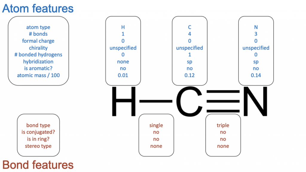
Figure 5. Graphical feature representation example input to the D-MPNN. A feature vector is assigned to each atom/node and bond/edge.
The model employed in the paper is a Directed Message Passing Neural Network (D-MPNN)4, which is a type of graph convolutional neural network. As its name suggests, graph convolutional neural networks act directly on graph structures, which includes chemical structures. Unlike fingerprint representation, which assigns a single fixed-length feature vector to a molecule, graphical representation assigns a feature vector to each bond and atom in a chemical structure (Figure 5).
I won’t go over the D-MPNN algorithm in complete detail, but you can find more information here4. Briefly, the D-MPNN can be understood as a multistep neural network. Each step is essentially a feedforward neural network that generates a set of hidden representations that are used as inputs for the next step. At the core of the D-MPNN is the message passing step, which takes advantage of the local substructures of the molecule graph to update hidden vectors (Figure 6). After the message passing step, hidden vectors from all edges are summed together into a single fixed-length hidden vector, which is fed into a feedforward neural network to yield the prediction, similar to the Morgan fingerprint approach above. This summation, often referred to as pooling, is a common strategy in deep learning to efficiently handle variable sized input samples.
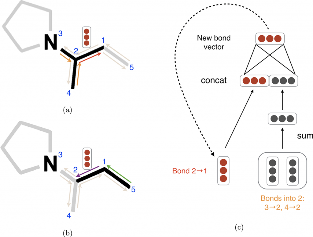
Figure 6. Illustration of bond-level message passing in the D-MPNN. Each bond is represented by a pair of directed edges. (a) Messages from the orange directed bonds are used to inform the update to the hidden state of the red directed bond. (b) Similarly, a message from the green bond informs the update to the hidden state of the purple directed bond. (c) Illustration of the update function to the hidden representation of the red directed bond from diagram (a). This message passing is an iterative process that can be repeated multiple times (typically 5).
My experience with using chemprop
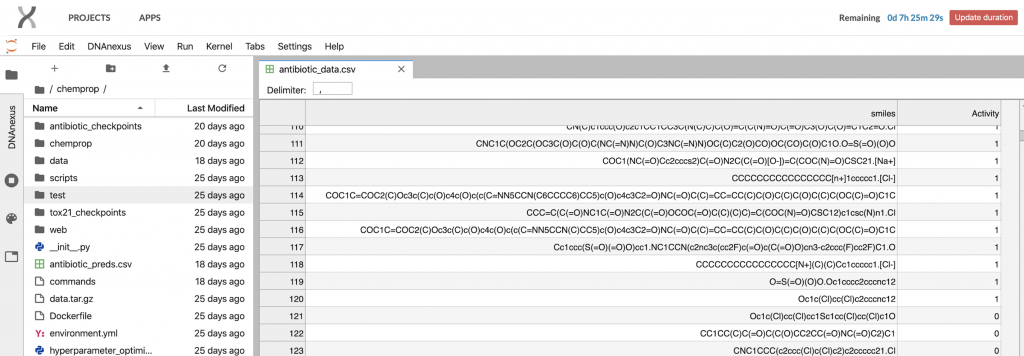
Figure 7. Screenshot of JupyterLab interface running on the DNAnexus Platform. A csv table of input data for chemprop is displayed.
The D-MPNN used by the authors is conveniently implemented in a package, chemprop, which is available on Github. It is recommended that chemprop is installed on a system with a CUDA GPU in order to make training significantly faster. Thankfully, the DNAnexus Platform provides JupyterLab sessions running on AWS GPU instances that make installing and running chemprop fairly straightforward, especially for those with basic python and command line experience (Figure 7). To get model training working, chemprop only requires a csv file containing molecules (as SMILES strings) and known target values. I was able to get their code working and train a model in under an hour on a DNAnexus mem3_ssd1_gpu_x8 instance, which is comparable to a AWS P3 instance.
Here’s the command I used to reproduce their training as best I can:
python train.py --data_path data/antibiotic_data.csv --dataset_type classification --save_dir antibiotic_checkpoints --depth 5 --hidden_size 1600 --dropout 0.35 --features_generator rdkit_2d_normalized --no_features_scaling --ffn_num_layers 1 --ensemble 20I used my trained model to predict the antibiotic activity of halicin and the eight other molecules Stokes et al. experimentally validated to show antibiotic activity. Admittedly, the results are a bit mixed compared to the predictions reported by Stokes et al. (Table 1). I’m guessing this is because the training set they provide consists of 2,560 molecules, of which only 120 are positive for antibiotic activity, which is very small compared to the number of free parameters in the model (5.6 million). At this scale, complex models like neural networks suffer from overfitting in the bias-variance tradeoff problem, where small changes in the data or model can lead to drastically different results.
Table 1. Comparison of predictions for halicin and the eight other novel molecules experimentally validated to show antibiotic activity.
| Name or ZINC ID | SMILES | My prediction | Stokes et al.’s prediction |
| Halicin | C1=C(SC(=N1)SC2=NN=C(S2)N)[N+](=O)[O-] | 0.4331186 | 0.331534501 |
| ZINC000098210492 | COC(=O)c1cc(F)c(N2CCN(C)CC2)cc1F | 0.95579629 | 0.97141532 |
| ZINC000001735150 | O=C1CSC(=S)N1/N=C/c1ccc([N+](=O)[O-])s1 | 0.62340529 | 0.941529986 |
| ZINC000225434673 | O=[N+]([O-])C(Br)(Br)/[N+](O)=N/c1nonc1/N=N\c1nonc1/N=[N+](\O)C(Br)(Br)[N+](=O)[O-] | 0.09552826 | 0.881357093 |
| ZINC000019771150 | CN1CCN(/N=C/c2ccc([N+](=O)[O-])s2)CC1 | 0.56568499 | 0.874699378 |
| ZINC000004481415 | N=C1[C@@H](C(N)=O)SC(=S)N1/N=C(\N)S | 0.58606944 | 0.872656737 |
| ZINC000004623615 | C[C@@H]1CN(c2cc(N)c([N+](=O)[O-])cc2F)C[C@H](C)N1 | 0.8500762 | 0.870749618 |
| ZINC000238901709 | CN1N[C@H](c2cccs2)[C@H]2C(=O)NC(=O)[C@H]21 | 0.19579908 | 0.857387473 |
| ZINC000100032716 | C[C@H]1CN(c2cc3c(cc2[N+](=O)[O-])c(=O)c(C(=O)O)cn3C2CC2)CCN1/N=N/c1ccc(S(N)(=O)=O)cc1 | 0.54675352 | 0.850668466 |
While not particularly well-advertised, the chemprop code also includes a rationale feature for interpretability that identifies the chemical substructure responsible for a positive predictive value. I was really excited to use this option to learn why some of these novel antibiotics are able to do what they do, but the interpretation feature only returns an answer for molecules that exceed the prediction threshold of 0.5 (Table 2); by chemprop’s own admission, halicin should be predicted to not have any antibiotic activity.
Table 2. Example of chemprop’s rationale interpretation output for a model that predicts toxicity. When a molecule is predicted to be non-toxic (prediction < 0.5), a rationale for prediction is not provided.
| SMILES | Predicted toxicity | Rationale | Rationale score |
| O=N+c1cc(C(F)(F)F)cc(N+[O-])c1Cl | 0.014 | NONE | NONE |
| C[C@]12CC@H[C@H]3C@@H[C@@H]1CC[C@]2(O)C(=O)COP(=O)([O-])[O-] | 0.957 | C1C[CH2:1][C:1][C@@H]2[C@@H]1[C@@H]1CC[C:1][C:1]1C[CH2:1]2 | 0.532 |
Final thoughts
As it stands now, while promising, my opinion is that the D-MPNN method suffers too greatly from the problem of overfitting to be useful for production. The most straightforward way to resolve this issue is to gather more data. This is not a problem entirely unique to molecular property prediction, but depending on the application, gathering more data can be either trivial or very costly. Given the rarity of known antibiotics, I’d imagine that gathering substantially more positive examples for training would be borderline impossible. Within the deep learning community, several techniques have been developed to maximize the performance of neural networks with smaller datasets. One such technique is transfer learning, which is a method where a model developed for a task is reused as the starting point for a model on a second task. Another promising technique is semi-supervised learning, which augments a small labeled set of training instances with a larger unlabeled set. The vast multitude of organic and biomolecules in databases easily provides more than enough unlabeled data. Finally, there is active learning, where the learning algorithm selects which of the unlabeled examples it wants labeled. In fact, a form of active learning is somewhat touched upon in the Stokes et al paper when they used different iterations of their model to comb a dataset for potential antibiotics, experimentally validate these molecules, and add the newly labeled data for the next iteration of training.
In yet another twist of events, the drug halicin, which was championed in the paper as a novel antibiotic, may not be as novel as originally thought. As reported by Chemical & Engineering News: “An unpublished 2017 study also identified this molecule’s antibiotic activity, but those researchers chose not to pursue it because of its similarity to a compound that the US Food and Drug Administration was already evaluating. Jonathan M. Stokes of Broad Institute of MIT and Harvard who is a coauthor of the new study says the group was not aware of the 2017 research until March 2.”5
Despite my suggestions and criticisms, however, I believe chemprop and the D-MPNN are steps in the right direction for cheminformatics and machine learning. In my opinion, this study represents the cleanest approach to deep learning in chemistry and drug development at the moment. In fact, I would like to see the D-MPNN applied to other applications involving graphs, such as graph genomes. It also helps that chemprop is relatively easy and quick to run, requiring very little knowledge of machine learning or chemistry to get working. This will surely encourage others to try it out and see what they can do with it.
References
- Stokes, Jonathan M., et al. “A deep learning approach to antibiotic discovery.” Cell 180.4 (2020): 688-702.
- Conly, J. M., and B. L. Johnston. “Where are all the new antibiotics? The new antibiotic paradox.” Canadian Journal of Infectious Diseases and Medical Microbiology 16.3 (2005): 159-160.
- Rogers, David, and Mathew Hahn. “Extended-connectivity fingerprints.” Journal of chemical information and modeling 50.5 (2010): 742-754.
- Yang, Kevin, et al. “Analyzing learned molecular representations for property prediction.” Journal of chemical information and modeling 59.8 (2019): 3370-3388.
- https://cen.acs.org/physical-chemistry/computational-chemistry/AI-finds-molecules-kill-bacteria/98/web/2020/02?utm_source=Twitter&utm_medium=Social&utm_campaign=CEN